Fixed, variable and gross costs. Average cost

The concept of average costs. Average fixed costs (AFC), average variable costs (AVC), average total costs (ATC), the concept of marginal cost (MC) and their schedules.

Average cost is the value of the total costs attributable to the value of the product produced.

Average costs are further divided into average fixed costs and average variable costs.

Average fixed costs(AFC) is the amount of fixed costs per unit of output.

Average variable costs(AVC) is the value variable costs per unit of production.

Unlike average fixed costs, average variable costs can both decrease and increase as output increases, which is explained by the dependence of total variable costs on output. Average variable costs reach their minimum at the volume that provides the maximum value of the average product

Average total cost(ATC) is the total cost of production per unit of output.

ATC = TC/Q = FC+VC/Q

marginal cost is the increase in total costs caused by an increase in output per unit of output.

Curve MC intersects AVC and ATC at points corresponding to the minimum value of the average variables and average total costs.

Question 23. Production costs in the long run. Depreciation and amortization. The main directions of use of depreciation funds.

The main feature of costs in the long run is the fact that they are all variable - the firm can increase or decrease capacity, and it also has enough time to decide to leave this market or enter it from another industry. Therefore, in the long run, they do not single out average fixed and average variable costs, but analyze the average cost per unit of output (LATC), which in essence are both average variable costs.

Depreciation of fixed assets (funds ) - decrease in the initial cost of fixed assets as a result of their wear and tear in the production process (physical wear) or due to the obsolescence of machines, as well as a decrease in the cost of production in the context of increased labor productivity. Physical deterioration fixed assets depends on the quality of fixed assets, their technical improvement (design, type and quality of materials); features of the technological process (speed and cutting force, feed, etc.); the time of their action (number of days of work per year, shifts per day, hours of work per shift); degree of protection from external conditions (heat, cold, humidity); the quality of care for fixed assets and their maintenance, from the qualifications of workers.

Obsolescence- decrease in the cost of fixed assets as a result of: 1) a decrease in the cost of production of the same product; 2) the emergence of more advanced and productive machines. The obsolescence of means of labor means that they are physically suitable, but do not justify themselves economically. This depreciation of fixed assets does not depend on their physical depreciation. A physically fit machine can be so morally obsolete that its operation becomes economically unprofitable. Both physical and moral deterioration leads to a loss of value. Therefore, each enterprise should ensure the accumulation of funds (sources) necessary for the acquisition and restoration of finally depreciated fixed assets. Depreciation(from the middle - century. lat. amortisatio - redemption) is: 1) the gradual depreciation of funds (equipment, buildings, structures) and the transfer of their value in parts to manufactured products; 2) decrease in the value of taxable property (by the amount of capitalized tax). Depreciation is due to the peculiarities of the participation of fixed assets in the production process. Fixed assets are involved in the production process a long period(at least one year). At the same time, they retain their natural shape, but gradually wear out. Depreciation is charged monthly at the established rates depreciation charges. The accrued depreciation amounts are included in the cost of products or distribution costs and at the same time, due to depreciation deductions, sinking fund, used for the complete restoration and overhaul of fixed assets. Therefore, proper planning and the actual calculation of depreciation contributes to the accurate calculation of the cost of production, as well as determining the sources and amounts of financing for capital investments and overhaul fixed assets. depreciable property recognized as property, results of intellectual activity and other objects of intellectual property that are owned by the taxpayer and are used by him to generate income and the cost of which is repaid by accruing depreciation. Depreciation deductions - accruals with subsequent deductions, reflecting the process of gradual transfer of the cost of labor instruments as they wear out and obsolescence to the cost of products, works and services produced with their help for the purpose of accumulation Money for a full recovery. They are accrued both on material assets (fixed assets, low-value and wearing items) and on intangible assets (intellectual property). Depreciation deductions are made according to established depreciation rates, their amount is set for a certain period for a specific type of fixed assets (group; subgroup) and is usually expressed as a percentage per year of depreciation to their book value. Sinking fund - a source of capital repairs of fixed assets, capital investments. Formed from depreciation charges. Depreciation task (depreciation) - to allocate the cost of durable tangible assets to costs over the expected life based on the application of systematic and rational records, i.e. it is a process of distribution, not evaluation. AT this definition there are several important points. First, all durable tangible assets other than land have a finite life. Due to the limited life of these assets, the cost of these assets must be allocated to costs over all the years of their operation. The two main reasons for the limited life of assets are depreciation and obsolescence (obsolescence). Periodic repairs and careful maintenance can keep buildings and equipment in good condition and greatly extend their life, but eventually every building and every machine must fall into disrepair. The need for depreciation cannot be eliminated by regular repairs. Obsolescence is the process by which assets do not meet modern requirements due to progress in the development of technology and for other reasons. Even buildings often become obsolete before they physically wear out. Second, depreciation is not a cost appraisal process. Even if the market price of a building or other asset may rise as a result of a good deal and specific market conditions, depreciation should still be accrued (accounted for), because it is a consequence of the allocation of previously incurred costs, and not a valuation. Determining the amount of depreciation for the reporting period depends on: the initial cost of objects; their salvage value; depreciable cost; expected useful life.

A manufacturing enterprise is created to manufacture certain products and make a profit when selling them. All costs that are incurred in production are called costs. In order to avoid losses, it is necessary to determine the volume of production, and how much money should be spent on its release. For this, average and marginal production costs are used.

Average production costs

When production grows, so do the costs of wages, raw materials, electricity, and so on, such costs are variable, since they depend on the quantity of output. At the start of production and small volumes of business, variable costs are insignificant, then the number of products increases, and the level of costs decreases, since there are savings on volumes. There are other costs that are constantly incurred, regardless of whether products are produced or not, even if there is no output of goods, fixed costs will be incurred. It can be rent payments, salaries of office employees, utility bills and more.

Variable and fixed costs are all costs spent on the production of a specific volume of goods. And when we talk about the cost per unit of production, this is the average cost. Average production costs are the costs per unit of output, which are calculated as a result of the ratio of total costs per unit of output. For example, a company produced five soft toys, spending 1500 rubles on it. This suggests that the average cost is 300 rubles and the cost of goods cannot be lower than this amount. But this does not mean that the same amount must be spent on the production of another unit of goods. To determine the desired volume of production, it is necessary to determine how much money is required for this. The marginal cost of producing a good is the cost of producing an additional unit of output. They show changes in costs that affect the change in production volumes.

Marginal cost of production

The definition of marginal production costs (MC from the English marginal product) is carried out according to the formula:

MC = Variable Cost Growth / Output Growth

For example, when there is an increase in sales per 100 pieces of goods, the company's costs will increase by 1000 rubles, while the marginal cost will be 1000 / 100 = 10 rubles. This suggests that an additional unit issued will cost 10 rubles.

The average and marginal costs of production are interconnected, a change in the ratio can serve as the basis for adjusting the volume of output. For example, if marginal costs are less than average, then output must be increased. If marginal costs are higher than average, then it is worth reducing production volumes.

The optimal ratio is when the marginal cost is equal to the minimum value of the average cost. AT this case do not increase production, as costs will increase.

When output increases, costs may change:

a) evenly, since in this case the marginal cost will be constant and equal to the variables per unit of output;

b) accelerated, when marginal cost rises with an increase in output. This may be due to the law of diminishing returns, or to the rising cost of variable costs;

c) slowly, when the cost of raw materials, materials and other costs decrease with the growth of output, while marginal costs are reduced.

Why does average variable cost increase as output increases? To answer this question economic theory uses the category of marginal cost.

Marginal (majority) costs (MC) reflect the increase in total costs caused by an increase in output per unit of output:

The value of marginal cost can be found as the first derivative of the total cost function:

So, marginal cost is the sum of the change in fixed costs per unit of change in output and the change in variable costs per unit of change in output. But after all, fixed costs do not change in the short run, that is:

And this means that marginal cost is, first of all, a change in variable costs in relation to a change in output per unit, that is:

There are important relationships between marginal, average total, and average variable costs. First of all, this concerns the relationship between MC and AVC. If the variable costs per unit of output are higher than marginal costs, then they decrease with each successive unit of output. In this case, if AVC becomes less than MC, then the value of AVC starts to increase. Therefore, equality occurs between these two types of costs when AVC takes a minimum value. The average total cost curve is the sum of the average fixed and average variable costs, and variable costs play a decisive role here. Therefore, the patterns characteristic of the relationship between VC and AVC are valid for MC and ATC. This means that the MC curve crosses the ATC at its minimum.

Marginal cost fully reflects the law of diminishing marginal returns of a factor of production. Since the productivity of each additional unit of a factor of production is less than the productivity of its previous unit, then the cost of attracting this additional unit turns out to be greater. Therefore, an increase in the volume of production associated with the involvement of additional units of production factors is accompanied by an increase in marginal costs. Up to a certain point, these increasing costs are offset by an increase in the total productivity of all units of the given factor used, which is accompanied by an increase in average returns and a decrease in average costs. However, this is only possible under the condition that the total productivity of a factor of production grows faster than the return on attracting each additional unit of this resource decreases, i.e. if average cost falls faster than marginal cost rises.

Therefore, the firm's decision to increase production is always preceded by a comparison of marginal and average costs. If marginal cost is below average, then the expansion of production will lead to a further decrease in average cost. If, on the other hand, marginal costs are greater than average, then average costs can only be reduced by reducing output. The minimum average cost is achieved when the average and marginal costs of production are equal. Accordingly, the moment of the most efficient allocation of resources within the firm is characterized by the achievement of a minimum level of average production costs.

Thus, the firm must monitor the formation of not only total, but also marginal and average costs, compare their movement with the dynamics of marginal and average products. And then production technology a firm can obtain an optimal structure that ensures the formation of minimum average production costs, high growth rates of marginal product, and a rapid decrease in marginal labor costs.

2.3.1. Production costs in a market economy.

production costs - It is the monetary cost of acquiring the factors of production used. Most cost effective method production is considered to be the one at which production costs are minimized. Production costs are measured in terms of costs incurred.

production costs - costs that are directly related to the production of goods.

Distribution costs - costs associated with the sale of manufactured products.

The economic essence of costs is based on the problem of limited resources and alternative use, i.e. application of resources in this production excludes the possibility of using it for another purpose.

The task of economists is to choose the most optimal use of factors of production and minimize costs.

Internal (implicit) costs - this is the cash income that the company donates, independently using its own resources, i.e. These are the returns that could be received by the firm for its own use of resources under the best of possible ways their applications. opportunity cost lost opportunity is the amount of money needed to divert a particular resource from the production of good B and use it to produce good A.

Thus, the costs in cash that the company has carried out in favor of suppliers (labor, services, fuel, raw materials) is called external (explicit) costs.

The division of costs into explicit and implicit there are two approaches to understanding the nature of costs.

1. Accounting approach: production costs should include all real, actual costs in cash (wages, rent, opportunity costs, raw materials, fuel, depreciation, social security contributions).

2. Economic approach: production costs should include not only actual costs in cash, but also unpaid costs; related to the missed opportunity for the most optimal use of these resources.

short term(SR) - the length of time during which some factors of production are constant, while others are variable.

Constant factors - the total size of buildings, structures, the number of machines and equipment, the number of firms that operate in the industry. Therefore, the possibility of free access of firms in the industry in the short run is limited. Variables - raw materials, the number of workers.

Long term(LR) is the length of time during which all factors of production are variable. Those. during this period, you can change the size of buildings, equipment, the number of firms. In this period, the firm can change all production parameters.

Cost classification

fixed costs (FC) - costs, the value of which in the short term does not change with an increase or decrease in production volume, i.e. they do not depend on the volume of output.

Example: building rent, equipment maintenance, administration salary.

C is the cost.

The fixed cost graph is a straight line parallel to the x-axis.

Average fixed costs (A F C) – fixed costs per unit of output and is determined by the formula: A.F.C. = FC/ Q

As Q increases, they decrease. This is called overhead allocation. They serve as an incentive for the firm to increase production.

The graph of average fixed costs is a curve that has a decreasing character, because as the volume of production increases, the total revenue grows, then the average fixed cost is an ever smaller amount that falls on a unit of products.

variable costs (VC) - costs, the value of which varies depending on the increase or decrease in the volume of production, i.e. they depend on the volume of output.

Example: the cost of raw materials, electricity, auxiliary materials, wages (workers). The bulk of the costs associated with the use of capital.

The graph is a curve proportional to the volume of output, which has an increasing character. But its nature can change. In the initial period, variable costs grow at a higher rate than the output. As the optimal size of production (Q 1) is reached, there is a relative saving of VC.

Average variable costs (AVC) – the amount of variable costs per unit of output. They are determined by the following formula: by dividing VC by the volume of output: AVC = VC/Q. First, the curve falls, then it is horizontal and sharply increases.

A graph is a curve that does not start from the origin. The general character of the curve is increasing. The technologically optimal output size is reached when AVCs become minimal (p. Q - 1).

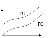
Total Costs (TC or C) – a set of fixed and variable costs of the firm, in connection with the production of products in the short run. They are determined by the formula: TC = FC + VC

Another formula (a function of the volume of production): TS = f (Q).

Depreciation and amortization

Wear is the gradual loss of value by capital resources.

Physical deterioration- loss of consumer qualities by means of labor, i.e. technical and production properties.

The decrease in the value of capital goods may not be associated with the loss of their consumer qualities, then they speak of obsolescence. It is due to an increase in the efficiency of production of capital goods, i.e. the emergence of similar, but cheaper new means of labor, performing similar functions, but more advanced.

Obsolescence is a consequence of scientific and technological progress, but for the company it turns into an increase in costs. Obsolescence refers to changes in fixed costs. Physical wear and tear - to variable costs. capital goods serve more than one year. Their value is transferred to finished products gradually as it wears out - this is called depreciation. Part of the proceeds for depreciation is formed in the depreciation fund.

Depreciation deductions:

Reflect the assessment of the amount of depreciation of capital resources, i.e. are one of the cost items;

Serves as a source of reproduction of capital goods.

The state legislates depreciation rates, i.e. the percentage of the value of capital goods by which they are considered depreciated in a year. It shows how many years the cost of fixed assets should be reimbursed.

Average total cost (ATC) – the sum of the total costs per unit of production:

ATC = TC/Q = (FC + VC)/Q = (FC/Q) + (VC/Q)

The curve is V-shaped. The output corresponding to the minimum average total cost is called the technological optimism point.

Marginal Cost (MC) – the increase in total costs caused by an increase in production by the next unit of output.

Determined by the following formula: MC = ∆TC/ ∆Q.

It can be seen that fixed costs do not affect the value of MC. And MC depends on the increment in VC associated with an increase or decrease in output (Q).

Marginal cost measures how much it will cost a firm to increase output per unit. They decisively influence the choice of the volume of production by the firm, since. this is exactly the indicator that the firm can influence.

The graph is similar to AVC. The MC curve intersects the ATC curve at the point corresponding to the minimum total cost.

In the short run, the company's costs are both fixed and variable. This follows from the fact that the company's production capacity remains unchanged and the dynamics of indicators is determined by the growth in equipment utilization.

Based on this graph, one can new schedule. Which allows you to visualize the capabilities of the company, maximize profits and view the boundaries of the existence of the company in general.

For the decision of the company, the most important characteristic is the average values, the average fixed costs fall as the volume of production increases.

Therefore, the dependence of variable costs on the function of production growth is considered.

At stage I, average variable costs decrease, and then begin to grow under the effect of economies of scale. For this period, it is necessary to determine the break-even point of production (TB).

TB is the level of physical volume of sales over the estimated period of time at which the proceeds from the sale of products coincide with production costs.

Point A - TB, where revenue (TR) = TS

Restrictions that must be observed when calculating TB

1. The volume of production is equal to the volume of sales.

2. Fixed costs are the same for any volume of production.

3. Variable costs change in proportion to the volume of production.

4. The price does not change during the period for which the TB is determined.

5. The price of a unit of production and the cost of a unit of resources remains constant.

Law of diminishing returns is not absolute, but relative, and it operates only in the short term, when at least one of the factors of production remains unchanged.

Law: with an increase in the use of one factor of production, while the rest remain unchanged, sooner or later a point is reached, starting from which the additional use of variable factors leads to a decrease in the increase in production.

The action of this law assumes the immutability of the state of technically and technologically production. And so technological progress can change the scope of this law.

The long run is characterized by the fact that the firm is able to change all the factors of production used. In this period variable nature of all applied factors of production allows the firm to use the most optimal options for their combination. This will be reflected in the magnitude and dynamics of average costs (costs per unit of output). If a firm decides to increase output, but initial stage(ATS) will first decrease, and then, when more and more new capacities are involved in production, they will begin to increase.

The graph of long-term total costs shows seven different options (1 - 7) for the behavior of ATS in the short term, since The long run is the sum of the short runs.

The long run cost curve consists of options called growth steps. In each stage (I - III) the firm operates in the short run. The dynamics of the long-run cost curve can be explained using scale effect. Change by the firm of the parameters of its activities, i.e. the transition from one version of the size of the enterprise to another is called change in the scale of production.

I - on this time interval, long-term costs decrease with an increase in the volume of output, i.e. there is economies of scale - a positive effect of scale (from 0 to Q 1).

II - (this is from Q 1 to Q 2), at this time interval of production, the long-term ATS does not react in any way to an increase in production, i.e. remains unchanged. And the firm will have constant returns to scale (constant returns to scale).

III - long-term ATS with an increase in output grow and there is a loss from the increase in the scale of production or negative scale effect(from Q 2 to Q 3).

3. AT general view profit is defined as the difference between total revenue and total costs for a certain period of time:

SP = TR –TS

TR ( total revenue) - the amount of cash receipts by the company from the sale of a certain amount of goods:

TR = P* Q

AR(average revenue) is the amount of cash receipts per unit of product sold.

Average revenue is equal to the market price:

AR = TR/ Q = PQ/ Q = P

MR(marginal revenue) is the increase in revenue that arises from the sale of the next unit of production. In the condition perfect competition it is equal to the market price:

MR = ∆ TR/∆ Q = ∆(PQ) /∆ Q =∆ P

In connection with the classification of costs into external (explicit) and internal (implicit) different concepts of profit are assumed.

Explicit costs (external) determined by the amount of expenses of the enterprise to pay for the purchased factors of production from the outside.

Implicit costs (internal) determined by the cost of resources owned by the enterprise.

If we subtract external costs from total revenue, we get accounting profit - takes into account external costs, but does not take into account internal ones.

If we subtract internal costs from accounting profit, we get economic profit.

Unlike accounting profit, economic profit takes into account both external and internal costs.

Normal profit appears in the case when the total revenue of an enterprise or firm is equal to the total costs, calculated as alternative. The minimum level of profitability is when it is profitable for an entrepreneur to do business. "0" - zero economic profit.

economic profit(net) - its presence means that resources are used more efficiently at this enterprise.

Accounting profit exceeds the economic one by the amount of implicit costs. Economic profit serves as a criterion for the success of the enterprise.

Its presence or absence is an incentive to attract additional resources or transfer them to other areas of use.

The purpose of the firm is to maximize profit, which is the difference between total revenue and total costs. Since both costs and income are a function of the volume of production, the main problem for the firm is to determine the optimal (best) volume of production. The firm will maximize profit at the level of output at which the difference between total revenue and total cost is greatest, or at the level at which marginal revenue equals marginal cost. If the firm's losses are less than its fixed costs, then the firm should continue to operate (in the short run), if the losses are greater than its fixed costs, then the firm should stop production.

In the classification of costs, in addition to fixed, variable and average, there is a category of marginal costs. All of them are interconnected, in order to determine the value of one type, it is necessary to know the indicator of another. So, marginal costs are calculated as a private increase in total costs and an increase in output. To minimize costs, that is, to achieve what each economic entity strives for, it is necessary to compare marginal and average costs. What conditions of these two indicators are optimal for the manufacturer will be discussed in this article.

Types of costs

In the short term, when the impact of economic factors can be realistically foreseen, a distinction is made between fixed and variable costs. They are easy to classify, since the variables change with the volume of output of goods, but the constants do not. Expenses associated with the operation of buildings, equipment; the salary management personnel; payment of watchmen, cleaners is a monetary cost of resources that make up fixed costs. Whether the enterprise produces products or not, they still have to pay monthly.

The wages of the main workers, raw materials and materials are the resources that make up the variable factors of production. They vary depending on the output.

Total costs are the sum of fixed and variable costs. Average cost is the amount of money spent on the production of one unit of a good.

Marginal cost measures the amount of money that must be spent to increase output by one unit.

marginal cost chart

The graph shows two types of cost curves: marginal and average. The intersection point of the two functions is the minimum average cost. This is no coincidence, since these costs are interconnected. Average cost is the sum of average fixed and variable costs. Fixed costs do not depend on the volume of production, and when considering marginal costs, their change with an increase / decrease in volume is of interest. Therefore, marginal cost implies an increase in variable costs. This implies that the average and marginal costs must be compared with each other when finding the optimal volume.

It can be seen from the graph that marginal costs begin to increase faster than average costs. That is, average costs are still decreasing with volume growth, while marginal costs have already crept up.

Balance point

Turning our attention once again to the graph, we can conclude:

• The AC is located above the MC, since it is a large value, including, in addition to variables and fixed costs. While MC consists of an increase in only variable costs.
• The previous fact explains the right location of the AS relative to the MS. This is because per unit of volume growth, MC contains the difference in variable costs, and average costs (AC), in addition to variables, also include fixed costs.
• After the intersection of the functions at the minimum point, there is an increase in the costs of the marginal nature faster than the average ones. In this case, production becomes unprofitable.

The firm's equilibrium point in the market is optimal size production, in which the economic entity receives a stable income. The value of this volume is equal to the intersection of the MC curves with AS at the minimum value of AS.

Comparison of AC and MS

When the marginal incremental cost is less than the average cost, it makes sense for the firm's top managers to decide to increase production.

When these two quantities are equal, equilibrium is reached in the volume of output.

It is worth stopping the increase in output when the value of MC is reached, which will be higher than AC.

Average costs in the long run

All costs in the long run have a variable property. The firm, which has reached the level at which average costs begin to rise in the long run, is forced to begin to change the factors of production, which had previously remained unchanged. It turns out that the total average costs are identical to the average variables.

The curve of average costs in the long run is a line contiguous at the minimum points of the curves of variable costs. The graph is shown in the figure. At point Q2, the minimum cost is reached, and then it is necessary to observe: if there is a negative effect of scale, which rarely occurs in practice, then it is necessary to stop the increase in output at the volume in Q2.

Marginal income MP

An alternative approach in modern market economy to determine the volume of production at which costs will be minimal and profit - maximum, is to compare the values ​​of the marginal values ​​of income and costs.

Marginal revenue is the increase in cash that a company receives from an additional unit of output sold.

Comparing the amounts that each additionally introduced unit of output adds to gross costs and gross income, it is possible to determine the point of profit maximization and cost minimization, expressed by finding the optimal volume.

Analytical comparison of MS and MR

For example, the fictitious data of the analyzed company are presented below.

Table 1

Each unit of volume corresponds to a market price, which decreases as supply increases. The income generated by the sale of each unit of output is determined by the product of the volume of output and the price. Gross costs rise with each additional unit of output. Profit is determined after deducting all costs from gross income. Limit values income and costs are calculated as the difference between the corresponding gross values ​​from the increase in production volume.

Comparing the last two columns of the table, it is concluded that in the production of goods from 1 to 6 units, marginal costs are covered by income, and then their growth is traced. Even with the release of goods in the amount of 6 units, maximum profit is achieved. Therefore, after the firm increases the production of goods to 6 units, it will not be profitable for it to increase it further.

Graphical comparison of MS and MR

When graphical determination of the optimal volume, the following conditions are characteristic:

• Marginal revenue over cost - expansion of production.
• The equality of values ​​determines the equilibrium point at which the maximum profit is achieved. The production output becomes stable.
• The marginal cost of production exceeds the marginal revenue in magnitude - a sign of unprofitable output at a loss to the firm.

Marginal cost theory

In order for an economic entity to make a decision to increase the volume of production, such an economic tool as a comparison of marginal costs with average costs and marginal income comes to the rescue.

If, in the usual sense, costs are the costs of output, then the marginal type of these costs is the amount of money that must be invested in production in order to increase output by an additional unit. When output is reduced, marginal cost indicates the amount of money that can be saved.